PoMM User Manual
Module Overview
Purpose of the Policy Making Module
The objective of the Policy-Making Module (PoMM) is to enable users to analyze the impact of changes in the policies related to the adoption of NBS (or hybrid NBS) for mitigation of CECs from urban runoff, hence enabling users on both science and policy sides to devise what changes would be more effective.
In order to link the PoMM to real-world applications, this general objective has been declined into three specific objectives (or Central policy issues, CPIs) that allow decision-makers to explore, in a given context, the best ways
- to include NBSs among customary or preferred solutions in spatial planning;
- to include CECs in water monitoring plans;
- to develop a pilot management plan of CECs from urban runoff that includes NBS solutions.
To make all this possible the PoMM hinges on three pivots:
- Knowledge representation,
- Policy / decision case definition (mapping of case playground),
- Questioning, analysis of the outcomes of modelling/simulations, reporting for decision.
Who is the PoMM intended for
The PoMM is specially conceived for decision-makers and policy-makers who are involved (or might be involved) in the formation of policies and rulemaking about the adoption of NBS for the mitigation of runoff CECs.
Intended users of the PoMM include:
- Policymakers-rulemakers at town, province, regional level
- Bureaucratic and administrative agents (including controlling and permitting bodies)
- Politicians
- Planners
- Scientists.
From the PoMM viewpoint, user categories are not linked to the actual role played by a user in real-life (a user can play any role, real or fictional). Having this in mind, the PoMM is applicable to both actual and potential situations.
Key functionalities
The key functionalities of the PoMM module are described in the following table:
| Submodule/Functionality | Description |
|---|---|
| Knowledge representation | includes the terminology service which assures a common understanding across all PoMM parts, the information stored about the cases under study, and the guidelines for the different types of experiments |
| Policy / decision case definition (mapping of case playground) | includes the tools to describe the case under study in which PoMM experiments take place, to formalize the existing decision-making and policy-making procedures, information flows, and practices following the Business Process Model and Notation (BPMN), and to assign NUTS, NBS and CECs considered. |
| Questioning, analysis and reporting for decision support | includes the tools and interfaces to transform a research question into a PoMM query by designing experiments, then analyzing the outputs obtained. Reporting encompasses the tools to communicate the results in ways suitable for the intended targets. |
How to access the PoMM
You can access the PoMM module via the AI-DSS Platform following general login instructions and pressing the appropriate link on the platform's side menu.
User System / Device requirements
For optimal performance, the following hardware and operating system configurations are recommended:
- Operating System:
- 64-bit Windows 11, macOS Ventura, or latest Linux distributions
- Processor:
- Quad-core CPU (Intel i5/i7 or AMD Ryzen 5+)
- RAM:
- 8 GB or more
- Web Browser:
- Latest version of Chrome or Firefox (for best compatibility and speed)
- Display:
- 1080p (Full HD) or higher resolution
- No installation is needed.
- NetLogo Web does not support all features available in the desktop version of NetLogo. For advanced functionalities, consider installing the desktop version.
When using the PoMM, it is very important that you do not use the back/forward buttons of the browser as you run the risk of compromising your session and having to start over: just use the buttons and links that appear in the interface.
A matter of privacy

After following the link on the platform's side menu to access the module, you are asked again to accept a specific privacy policy concerning your information and its handling in the PoMM [Fig. 1].
The PoMM does not store user data, including uploaded files, configurations, models, simulations, or reports, beyond the duration of the active session. Once the session ends, all data will be permanently deleted from the platform's servers.
It is your sole responsibility to download and securely save any data, reports, or configurations generated or uploaded during the session. The PoMM is not liable for any loss of data due to failure to download or save session outputs.
While the PoMM platform implements standard security measures to protect active session data, users are advised to avoid uploading sensitive or confidential information.
If you do not agree to the policy conditions, you are redirected to the public area of the Help section of the module.
Strike the right button
The PoMM offers a wide variety of specific features all geared towards making your journey as satisfying and useful as possible.
It is important to strike the right button to start with! [Fig. 2]

- Start New Session: Begin a new policy modelling session from scratch.
- Restore Session: Resume a previously saved modelling session.
- Process templates: Decide your strategy by answering some questions to start a new session with a pre-configured process template.
- Agents simulation: Proceed with the Agent Based Simulation.
- Thesaurus & Vocabulary: Access the standardized terminology and definitions.
- Help & User's Guide: Access comprehensive documentation and user guides.
Brief flow of operations
The flow that users follow in the PoMM goes through 5 main steps:
- description of the case under study defining what the starting experimental context looks like with respect to the objectives to investigate (i.e.: to include NBSs among customary or preferred solutions in spatial planning; to include CECs in water monitoring plans; to develop a pilot management plan of CECs from urban runoff that includes NBS solutions)
- definition of an intervention to influence the baseline context in order to facilitate the achievement of one's goal (where should/can I act? how?)
- analysis of the outcomes of the experiment performed (how does the hypothesis of intervention change my initial context? what are the results obtained? am I closer to my goal?)
- documentation and sharing of results (how do I document and share the results of my experiment with other interested stakeholders?)
- overcoming doubts and obstacles in experimentation (what tools do I have to deepen and reduce the risk of language ambiguity/equivocality across different knowledge domains and fields of practice involved in my experiment?).
Difference between network modelling and agent-based modelling
There are two main modelling approaches in the PoMM:
- a network modelling approach to mapping out the relationships among variables that affect CEC-NBS decisions in a real-world procedural decision-making process to reveal the overall structure of the system, observe how the system behaves without any intervention, define what are the interventions needed to change the final state of the system to own advantage;
- an agent-based modelling approach simulating the actions and interactions of individual "agents" (could be different stakeholders but also for NBS solutions) within the system to explore what behaviour could emerge as a response to pollution risks, floodings, etc. It's like creating a virtual world where watching how individual behaviors add up to create larger and complex patterns.
By combining them, users can create models that are both cognitively realistic and dynamically rich and this is particularly valuable for studying complex systems, as in the case of the use of NBS solutions to mitigate the pollution effects of CEC contaminants from urban runoff phenomena.
The two modelling methods are managed separately in the PoMM, accessed from two different functions in the main menu that are not interconnected.
In a logical sense, networking modelling takes place ‘before’ the agent based modelling.
That is because the network modelling approach provides the "cognitive" framework, the understanding of how factors interrelate and helps to decide where to intervene.
The ABM approach provides the "behavioral" framework, the simulation of how agents act, and allows to explore and compare the sentiment and social response to NBS for CECs depending on factors like front and maintenance cost, risk-mitigating capacity, etc.
In PoMM you can choose which modelling system you want to use: you can use both if you want to get the best out of your analysis.
But you can also decide to use only one because you consider it more suitable for the type of reflections you are making.
Furthermore, both modelling techniques allow you to choose your own approach: are you interested in a purely descriptive or observational approach to gain a better understanding? Or are you interested in an approach that involves intervening on what you are observing and understanding the effects of your intervention? Are you interested in evaluating the impact of any changes following your intervention hypotheses? And from what point of view?
The PoMM allows you to do all this: read the following suggestions and user instructions very carefully to find your winning strategy!
Knowledge representation
The first pivot of the PoMM module is knowledge representation.
Activities like CEC characterization, NBS classification, policy-making guidelines intersect on the same case from different perspectives and with diverse vocabularies.
Sometimes the meaning of important terms that we use are confusing (multiple meanings depending on context or user, or synonyms) or a term is authoritatively defined somewhere, but its definition does not fit well with our shared domain.
We aimed to create clear, machine-readable definitions for key terms, establishing logical connections within the PoMM framework and simulations. This minimizes misunderstandings caused by differing interpretations of language across the various fields involved in D4Runoff.
Terminology (vocabulary, thesaurus and ontology)
The D4Runoff Thesaurs is a controlled and structured vocabulary, related to the domain the project deals with in, which concepts are represented by terms, organized so that relationships between concepts are made explicit.
The D4Runoff Thesaurus:

- Ensures everyone understands the information structure (common meaning).
- Clearly states the assumptions made about the subject.
- Checks that the subject information is consistent (verifies accuracy).
- Allows the subject information to be used again in different ways.
- Separates subject knowledge from how it's used.
- Simplifies searches and makes it easier to find information.
You can access the Thesaurus by simply clicking on the button on the main menu: a new browser window will open, allowing you to have the main definitions at your fingertips so that you can better understand how to design your case study [Fig. 3].
You do not need to authenticate to the Thesaurus if you are already logged in to the platform.

What you can do
The use of the vocabulary/thesaurus is very intuitive.
On the main page [Fig. 4] you can find:
- a bar on which to write the term you want to search for
- an alphabetical list on which you can click to search
- a list of main contents at your immediate disposal that help you understand some of the most relevant elements which represent the scope of analysis of the PoMM or are useful for your experiments
- a link to an advanced search.
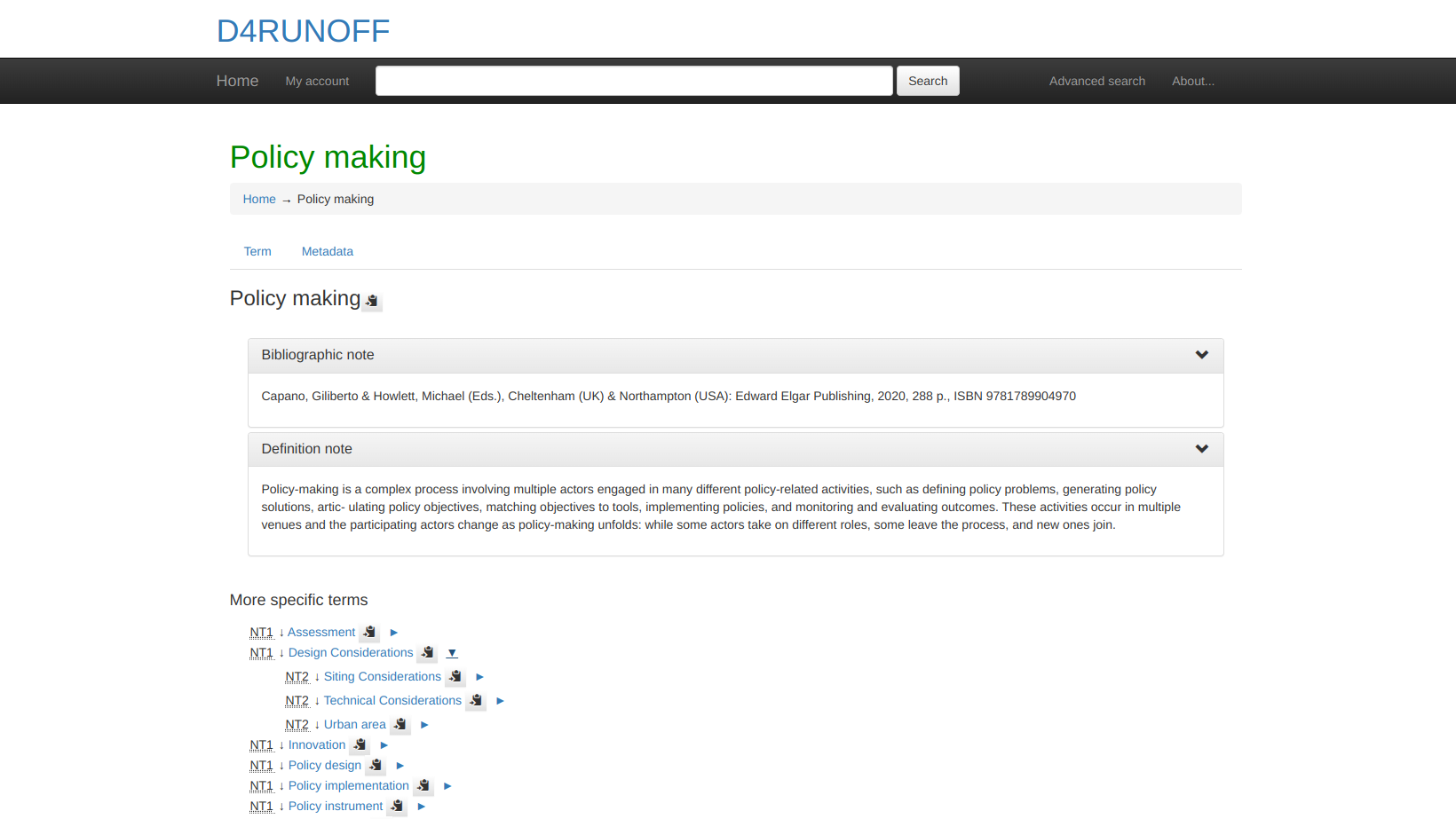
Fig. 5 - Example of a concept of the Thesaurus and its relationship

Note that the "My Account link" on the navigating bar is only available to system administrators.
The interface [Fig. 5] allows you to:
- see the description of each search term
- read definitions and bibliographical notes
- directly access other terms related to the entry you searched with more specific, broader, equivalent, preferred or semantically related meaning.
Note that the interface is multilingual but the contents are in English.
In the same screen of a defined term, different kinds of relationships are displayed allowing you to move easily from one term to another via the different links.

There are different kind of relationships you can find in the D4Runoff thesaurus that can include:
- hierarchical relationships such as broader term (BT) and narrower term (NT). These terms denote relationships between the concepts (not the terms) and indicate whether a concept contains or is contained by another concept. Hierarchical relationships can be used to broaden and narrow a search effectively and ensure that narrower terms fall within the scope of the broader terms;
- equivalence relationships such USE and UF (Use For). They are used to denote equivalence between terms (not concepts) and to distinguish between preferred terms and their synonyms (a term, which has the same meaning or covers the same concept as another term or multiple terms) or quasi-synonyms (a term that does not usually have the same meaning as the preferred term but does in the context of a specific thesaurus) [Fig. 6];
- associative relationships such as related terms (RTs). They are used to indicate that different terms in a thesaurus are related in some way or have an overlapping scope. They thus allow users to expand their initial search into different aspects of the subject.

The advanced search [Fig. 7] allows you to navigate the Thesaurus also, for example, from the notes that have been associated with each term, doing your own free search.

The Thesaurus is linked to qualified sources and validated vocabularies
- EUROVOC: a multilingual thesaurus (controlled vocabulary) maintained by the Publications Office of the European Union, used by the European Parliament, the Publications Office of the European Union, the national and regional parliaments in Europe, some national government departments, and other European organisations [Fig. 8]
- AGROVOC: a multilingual controlled vocabulary covering all areas of interest of the Food and Agriculture Organization of the United Nations (FAO), including food, nutrition, agriculture, fisheries, forestry and the environment.
- GEMET - GEneral Multilingual Environmental Thesaurus: a source of common and relevant terminology used under the ever-growing environmental agenda that has been developed since 1995 as an indexing, retrieval and control tool for the European Topic Centre on Catalogue of Data Sources (ETC/CDS) and the European Environment Agency (EEA), Copenhagen.
- EARTh - Environmental Applications Reference Thesaurus: represents a general- purpose thesaurus for the environment. It promises to become a core tool for indexing and discovering environmental resources by refining and extending GEMET.
Knowledge repository
The PoMM knowledge repository (help, user's manuals, technical documentation) has been organised as a semantic-rich website.
It was based on f the Mediawiki platform, an extremely powerful and scalable software, which enables the implementation of feature-rich wikis and allows you to move freely between contents depending on your qualification as a user. [Fig. 9]
What you can do
On the main page, you can access the main content and information.

From this page it is possible to reach every area of the help feature.
If you are a registered user (from the AI platform), you can access a restricted area that contains the Comprehensive Knowledge Base and Full Documentation and allows to:
- access the FAQ system and specific tutorials
- analyse case studies (including D4Runoff pilot sites) and applications of the PoMM in other contexts
- deepen the policy scenario
- deepen the underlying principles, mechanisms, and technology choices incorporating the theoretical body of knowledge that supports PoMM operations
- access targeted bibliographies and other useful resources
- access technical documentation about the technology, architecture, core modules and interconnections.
You will find a contextual help button all along your path in using the PoMM that can refer you to the appropriate sections in the Mediawiki platform.
Policy / decision case definition
In the PoMM, you build policy scenarios to map out the steps involved in making decisions that affect well focused central issues in order to operationalise the exploration, design and analysis of changes in the policies related to the adoption of NBS for mitigation of CECs from urban runoff.
Upstream of the activities for which the platform can offer support in your thinking, you should start by formulating your "research question" and keep it in mind all along the way: what are you trying to answer? What do you want to explore?
This step is fundamental to the entire PoMM process, serving as its core and ensuring the coherence and consistency of experiments and results.
Just to give you an idea of the type of questions on which you would like to reflect...:
- How can municipal procurement regulations be amended to effectively integrate NBS into the terms of reference for urban planning and design tenders?
- Within the existing municipal regulatory framework, which department—urban planning or public works—offers the most effective point of intervention for promoting NBS adoption in routine roadside renovations?
- Given the current regional legal framework, at what stage in the decision-making process would political advocacy be most impactful in securing a bill that mandates a recurring budget for CECs monitoring?
- Which office holds the greatest influence in obstructing regulations aimed at making CECs management plans mandatory?
- Which proposed NBS regulation, “A” or “B,” will have better impact and be more viable?
- Considering the current regional legal framework, where within the decision-making hierarchy should political pressure be applied to successfully delegate runoff management to water utilities?
- ....
As you can easily imagine, all these questions bring with them the initial need to understand the boundaries of your system and how things work today in your context.
Essentially, it's a way to visualize "your world" in relation to the relevant policy-making cases as it is, to create the ‘laboratory’ of the experiment and to map the framework of the case under study.

Typically, the definition of the policy/decision case starts with network modelling.
Procedural description (network modelling) of the case
To outline your case you have to start a new session from scratch.
From the main menu choose |Start new session| [Fig. 10]
Outline the case under study
You will need to outline your case study by following the steps below.
(1) Defining the geographic boundaries of your physical system
Your context will change radically if you are involved in analysing policies acting at different territorial levels: the policy processes or stakeholders to be involved may also change greatly. The PoMM allows you to keep track of the territorial level at which you are reasoning.
| Select the NUTS level to which your analysis relates.
NUTS (stands for Nomenclature of Territorial Units for Statistics) are statistical codes to define a geographical area in the European Union. The NUTS system divides each EU country into three levels: NUTS 1 (Major socio-economic regions); NUTS 2 (Basic regions for the application of regional policies); NUTS 3: Small regions for specific diagnoses. [Fig. 11] |
 |
| You can change the NUTS map display level in the top right of the screen and then directly select your area from the map of Europe on the left of the screen.
You can zoom on the map for better resolution. [Fig. 12] |
 |
| Most PoMM analyses will be probably reflected in NUTS 2 or NUTS 3 level areas.
If you select NUTS 3 level, you can also choose Local administrative units (LAU) from the contextual drop-down menu. [Fig. 13] |
 |
| Once the NUTS/LAU is selected, confirm selection to set the LAU code, if needed. [Fig. 14] |  |
| Press |Next ->| to complete the geographical information. [Fig.015]
If you realise you have made a mistake, you can go back and change your choice clicking on |<- Back| . The geographical boundary of your system is now completed. |
 |
(2) Select the targeted Natural based solution
The same reflection made for the territorial dimension applies to the type of NBS solution you are investigating: again, not all solutions act on all territorial levels or require the same implementation or regulatory processes.
Also in this case the PoMM allows you to keep track of this in your simulation even though in this case the identification and evaluation of the NBS should have already been developed in other sections of the AI platform that are dedicated to this purpose.
| The definition of your case study should be linked to the choice of the NBSs you would like to apply: to investigate which NBS is right for you, you will have already used other areas of the AI platform. In this section of the module, you can select them to keep track of your starting framework.
However, if in your case study, you do not need to select an NBS, you can simply confirm your choice not to select it. [Fig. 16] |
 |
| Choose NBS from the drop-down menu and press on |Confirm selection|. [Fig. 17]
The candidate NBS solutions in the drop-down menu are those made available from the University of Cantabria on the AI platform in the solution library section. |
 |
| The system will display a brief description of the selected NBS: you can then either verify your choice. [Fig. 18]
Press |Next ->| to complete the NBS information. If you realise you have made a mistake, you can go back and change your choice clicking on |<- Back| returning to the NUTS choice screen. The NBS selection for your unit of analysis is now completed. |
 |
(3) Choose the targeted Contaminants of emerging concern (CEC)
The contaminants you are investigating are also related both to the NBS solutions you have chosen and to specific problems that equally may have to be considered in very different policy making processes.
Again, the PoMM allows you to keep track of them in your simulation of the CECs you have identified. As with NBSs, the identification of targeted CECs should already have been developed in other sections of the AI platform that are dedicated to this very purpose.
| Next step in defining your case study (or unit of analysis) is the choice of CECs: to investigate which CEC is more relevant in your case, you will have already used other areas of the AI platform. In this section of the module, you can select them to keep track of your starting framework. [Fig. 19] |  |
| Select family of CEC from the drop-down menu.
The target CECs are chosen from a list provided by D4RUNOFF Partners working on the topic on the AI platform in the CECs library section. If you want to refine your search, you can also select compounds or CAS from the drop-down menu. [Fig. 20]. Press on |Confirm selection|. |
 |
| If you realise you have made a mistake, you can go back and change your choice clicking on |<- Back| returning to the NBS choice screen. [Fig. 21].
Press |Next| to complete the CEC information. The CEC selection for your unit of analysis is now completed. |
 |

The system allows you to keep a note of the choices you have made, possibly adding your comments to have a written trace that will feed the reporting of your experiment. [Fig. 22]
You can also leave the proposed text unchanged in the dialogue box that appears, but we suggest that you use these spaces to make your notes.
The activity of modelling decision making processes and scenario setting is a complex activity that may also require interactions and comparisons between different actors. By doing so, you do not risk losing valuable information.
With this first three steps you have completed the Unity of analysis definition (NUTS, NBS & CEC)
To proceed to the next stage of your case study baseline press |Next|.
(4) Define the actual (current) decision workflow diagram
To be able to intervene in a decision-making process and understand where and how, it is necessary to describe it.
| In the PoMM, this description is done using an interface to represent the decision-making diagrams.
The notation used is the BPMN (Business Process Model and Notation). [Fig. 23] |
 |
| BPMN is a visual modelling language for process workflows. It is an open standard notation for graphical flowcharts that can be easily understood by all stakeholders. [Fig. 24].
In our case, the BPMN represents the end-to-end flow of a policy process. The notation makes it possible to coordinate the sequence of processes and messages flowing between different process participants in a set of related steps. Even using only the basic notations of the BPMN, you can describe all usual procedural steps in policy and decision making processes. |
 |
| Here you find some basic hints for using BPMN notation with the PoMM BPMN interface. [Fig. 25] |  |
| If you do not want to describe your process directly within the PoMM BPMN interface or you already have designed your BPMN diagram using your modelling software, you can use your saved file. Upload it simply dragging and dropping in the interface.
But please make it sure it is in a compatible format (that is *.bpmn) otherwise you'll get an error message. | |
| To facilitate this step, if you are not familiar with the BPMN diagram, you can also choose an easy route where you can use some ready-made templates.
In this case, you should start the outline of your case at the very beginning of your session from the main PoMM menu selecting the |Process Template| option instead of |Start new session| . [Fig. 26] |
 |
| You have to answer a short survey to select what are the central policy issue you will explore, defining what type of action (regulatory or operative) do you plan to carry out, and what is your policy decision framework (risk driven, value driven or return driven). [Fig. 27]
The system will take care of selecting the most suitable template based on the strategy you have chosen. Of course, this is an example, which is plausible but which you should then adjust according to your needs: your real situation may in fact be different from the one proposed. |
 |
| Then, after answering the survey, you proceed normally from step (1) Defining the geographic boundaries of your physical system to the initial setting as explained before. | |
| When you get to step (4) Define the actual (current) decision workflow diagram you will already find on the PoMM BPMN interface a ready-made template chosen based on your answers and pre-designed on a plausible similar case. [Fig. 28]
You can modify it to adapt it to your case, removing some steps, revising annotations, adding elements etc. |
 |
| Now you need to individuate which are the entities in your process you consider potentially interesting for the subsequent modelling and simulation of policy making and interventions on it.
Depending on the focus of your investigation, you will need to ask yourself, for example, which elements of the process you want to concentrate on and define the variables that best express them. For example, if you think you can influence a task in your process that is ‘holding public meetings’ (perhaps to discuss the inclusion of NBS solutions in current construction processes), the linked variable could be ‘the level or index of stakeholder and local community involvement’. [Fig. 29] The reason why this step is necessary is precisely to allow you to isolate, in the decision-making process, the network of relationships that you are most interested in investigating, in order to allow simulations to understand what further actions (in relation to those identified) you can take to achieve your objectives. If you opt for the |Process Template| option, you will find these elements already prepared in the templates and they can serve as an example to ease your analysis. |
 |
| For each selected entity (i.e. a task) you must add an annotation indicating what is the main variable associated to it. [Fig. 30]
Generally you will add annotations to some of the tasks that are present in your BPMN process. You can do this simply by using the small tool that appears when you pass the mouse over the ‘task’ object and then "add text annotation" and write the note. It will appear next to the task in square brackets. [Fig. 31] |
 |
| Taking care to choose and describe the variables in such a way that they can be measured in a minimum to maximum range: this method will help you a lot in the following steps of modelling.
The annotation of entities is a fundamental step, otherwise it will not be possible to define those that you want to deal with in the subsequent modelling and simulation network. To have a fairly rich and interesting simulation, we suggest you identify at least 7 variables connected to the different entities in your process diagram (it would be better between 7 and 12). Bear in mind that this step helps you to reflect in a very precise way on the case you are analysing, helping you a lot to outline the most interesting elements. |
 |
| If you annotated or modified a diagram (whether it is the diagram that you create directly in the interface, or the one that you modify starting from a loaded template or from one of your file that you have uploaded to the system) you must select the |NEXT| button [Fig. 32] and continue your simulation up to the next check point (see below: 5 - Identify the most important entities for the decision workflow) otherwise your annotations are permanently lost! |  |
(5) Identify the most important entities for the decision workflow
Once you have defined in the previous step the decision-making process involved as it currently is and having identified some entities to analyse and their variables, you will have to go through the last mile of this phase to have your first baseline report.
This involves selecting the variables that you defined in the BPMN in the form of annotations and that will be shown in an interface where you can decide which ones will be analysed in the simulation.
Note that if you haven't inserted any variables in your BPMN (in the form of an annotation) you won't be able to select any nodes and therefore won't be able to proceed with the simulation proposed by the PoMM.
| After clicking on |NEXT| from the BPMN interface, you will find yourself in the environment for identifying the variables you have focused on. They will appear in the form of clickable nodes that you can select.[Fig. 33] |  |
| The interface allows you to select each node that will appear on the map box: click to confirm your selection (the node turn red). [Fig. 34] |  |
| You can also select your nodes from the drop-down menu above the map box. [Fig. 35] |  |
| In any case, before proceeding further, check carefully which nodes you have selected.
Press the button |Next to checkpoint| to complete this first cycle and download the file package related to the outline of your case study. [Fig. 36] |
 |
| You can add your comments about the work you have done in outlining the decision-making process you want to intervene in and have identified your points of interest.
This will help you keep track of your reasoning and will flow into a report that you can share. [Fig. 37] After adding your comments push |NEXT|. |
 |
| Now you are asked to download the Intermediate Report of your Experiment that describes what you have done until now, to outline the case under study and set the boundaries of the experiment. [Fig. 38]
In addition, the work done will be saved so that you can restore your session if you need so. You must download the Intermediate Report and the back-up files to be allowed to the next step: this is a form of guarantee to prevent you from losing the data you have entered. Remember: the system does not automatically save them for privacy reasons. |
 |
| If you don't intend to continue with the analysis after this check point, by downloading the file package you can also restore the session in another moment deciding which of the phases to restore: from point 1, reloading your choice of NUTS, NBS, CEC; from point 2 reloading your BPMN diagramming file, from point 3 reloading your chosen entities and the notes you added at this checkpoint, allowing you to start again right where you left off and beginning the simulation.
To restore your file, if needed, access from the PoMM main menu on |Restore Session|. [Fig. 39] |
 |
| The *zip file you download at the Intermediate Report checkpoint contains 3 folders and a series of files necessary for the various restore phases. [Fig. 40] |  |
| A very simple interface will guide you through restoring them. [Fig. 41]
Please be careful! Upload the files gradually in the order in which they are requested by the interface. Once you have uploaded the first ones, you can proceed further in the restore by pressing |Continue to upload|. You can stop at the level where you intend to restore. |
 |
Bottom-up modelling (agent based) of the case
Outline the case for ABM exploration

The Agent simulation is a separate feature of the PoMM module, powered on netLogo Web application, which you can access through the main menu. [Fig. 42]
In this case, your interface will directly load a basic simulation model. This model was prepared as part of the D4Runoff project for the PoMM module.
This is an agent-based model simulating the adoption dynamics of NBS within an urban environment. It explores how citizens, property owners, and a dynamic public authority interact under risks from flooding and CECs pollution in urban runoff. The model focuses particularly on how different conditions and policy choices influence NBS uptake and its subsequent impact on mitigating pollution.
It invites users to test scenarios and reflect on QUESTIONS like:
- How do people respond to environmental risk?
- What role does public policy play in driving or hindering adaptation?
- Who benefits - and who might be left behind?
The model features realistic actors: citizens and property owners (both residential and commercial), a dynamic Public Authority, and environmental monitors. Each actor reacts to events like floods or pollution, but their responses depend on their economic means, experience, and social surroundings. For example, wealthier property owners may adopt NBS more readily, while citizens in risk-prone areas may petition the government or choose to relocate.
This raises QUESTIONS:
- Are current policy tools equitable?
- Do incentives and taxes encourage resilience in vulnerable areas?
Set in a virtual city represented by a spatial grid, the model considers how elevation, proximity to water, and stochastic environmental events shape local risk. Users can adjust a range of parameters - from the frequency and intensity of floods to the distribution of economic capacity among residents.
This flexibility helps explore QUESTIONS such as:
- How might more frequent extreme events alter risk perception?
- What happens when economic inequality increases?
- How sensitive should policies be to citizen pressure or environmental monitoring data?
Each simulated time period unfolds with agents updating their behaviors, supporting (or opposing) NBS, and influencing the environment. The Public Authority responds to trends over time - adjusting policies, budgets, and political orientation. The model helps users uncover the unintended consequences and feedback loops inherent in urban systems, suggesting relevant QUESTIONS like:
- If NBS are adopted mainly in wealthier zones, could this shift risk elsewhere?
- Does awareness-raising lead to meaningful action?
- What are the long-term outcomes of shifting between pro-environment and pro-development stances?
Outputs include intuitive visuals and graphs tracking key indicators like risk exposure, public sentiment toward NBS, environmental quality, and NBS adoption. These help planners and policymakers trace the impact of their hypothesized decisions over time and evaluate trade-offs.
The model is not meant to provide definitive answers - it is a space for reflection and testing, guiding users to ask sharper, more targeted questions about resilience, equity, and the governance of urban environmental risks and NBS policies.
The interface is a console from which all the necessary simulations can be carried out using a series of elements already present.
Assumptions and Limitations of the default model
Simplifications:
- The economic system uses an abstract 'capacity' metric; costs and benefits are relative.
- Social influence is modeled based on spatial proximity, not complex social networks.
- NBS are represented generically, without differentiating specific types or detailed ecological functions beyond risk reduction percentages.
- Public Authority decision-making follows programmed rules based on specific inputs, simplifying real-world political complexities.
- Agent behavior is rule-based and driven by defined thresholds and calculations.
- The spatial environment uses a regular grid, and risk propagation is based on simplified distance/elevation functions.
Limitations:
- The model doesn't include detailed representations of other urban infrastructure (e.g., grey infrastructure like drainage systems).
- Agent diversity is limited to the defined attributes; factors like age, education, or detailed psychological profiles are not included.
- The financial impact of NBS maintenance on owners is implicit (via decay) rather than explicitly modeled as an ongoing cost affecting their capacity.
- The model is largely closed; it doesn't account for external shocks like major economic changes or technological breakthroughs not represented by the stochastic events.
- The specific mathematical distributions used for event frequency (Poisson) and intensity (Log-Normal) are assumptions about the nature of these hazards.
Loading models from the PoMM library or from your own library


In addition to the default model that is loaded when you access this section of the PoMM, you can also load other models available in the library [Fig. 43], or models that you have saved on your repositories [Fig. 44].
The models in the library may be variants with a different interface (for example, different output variables may be plotted) or have different hard-wired values (parameters set directly in the code).
For this reason, it is always important to read the documentation available in the Model Info tab.
Also remember that the model code is always visible, so you can check or change the model according to your needs.
Before starting: How the default model works
Simulated System: the default model operates on a 2D grid representing a stylized urban area featuring land and water zones. This area is populated by citizens and property owners who face periodic flood and pollution events. The model incorporates the decision-making process for adopting NBS, the effectiveness of these solutions, the role of environmental monitoring (specifically for CECs), and the dynamic nature of a public authority whose policies adapt based on environmental conditions and public sentiment.
1. Key Agents and Their Behaviors
The model features several agent types and the environment itself:
Citizens:
- Characteristics: Possess varying levels of economic capacity (which can be distributed unequally), sentiment towards NBS adoption, memory of recent risk events, susceptibility to social influence from neighbors, and the potential to relocate. They experience risk based on their current location.
- Decisions/Actions: Regularly update their memory of risk events and adjust their NBS sentiment based on personal experience, memory, and the sentiment of nearby citizens (social influence). If risk exposure remains high and they have sufficient economic capacity, they might move to a less risky area. They can also petition the Public Authority if their perceived risk and memory are high. Citizens are subject to taxation by the Public Authority.
Owners (Residential & Commercial):
- Characteristics: Similar to citizens regarding economic capacity, NBS sentiment, memory, and risk exposure. They are categorized as either "residential" or "commercial".
- Decisions/Actions: Update memory and risk perception. Decide whether to invest in NBS. Residential owners base this decision on their sentiment, affordability (considering economic capacity and taxes), perceived risk and long-term financial outlook. Commercial owners use a Return on Investment (ROI) calculation, comparing expected damage reduction from NBS against its cost. This is reflected in a willingness to pay for NBS (WTP) and in a willingness to take risks (WTA). Wealthier owners might expand their property holdings if their economic capacity stays high for a period. Owners are also subject to taxation.
Public Authority:
- Characteristics: A single agent representing the governing body. It manages a budget funded by taxes. Key dynamic attributes include its political alignment (shifting between pro-environment and pro-development stances), the strength of its policies, and its influence. It receives petitions from citizens expressing concern.
- Decisions/Actions: Periodically (monthly) adjusts its political alignment, policy strength, and influence based on factors like average citizen risk perception, average water contamination levels, the volume of citizen petitions, and its current budget balance. Annually, it sets the taxation rate based on its alignment and policy strength, then collects taxes from citizens and owners. If its budget allows and alignment is favorable, it may offer subsidies to owners in high-risk areas to encourage NBS adoption.
CEC Monitors:
- Characteristics: Stationary agents placed within water bodies. They have attributes defining their detection accuracy (related to a 'cost barrier'), their influence strength (for awareness campaigns), and their capacity to directly mitigate pollution.
- Decisions/Actions: Monitor local water for CECs. If high levels are detected, they can directly reduce some contamination based on their capacity. They can also trigger public awareness campaigns (boosting citizen/owner NBS sentiment) when contamination is high, although this effect is rate-limited across all monitors.
NBS Solutions:
- Characteristics: Represent specific NBS installations owned by an owner agent. Defined by cost, activation time (time to become effective), mitigation effectiveness (for flood and pollution), maintenance cost, radius of effect, age, and a decay rate representing diminishing effectiveness over time.
- Decisions/Actions: Once adopted by an owner, they take time to reach full effectiveness. They reduce flood and pollution risk within their designated radius. Their effectiveness decreases over time unless maintained (maintenance is assumed to be funded by the owner, impacting their implicit finances rather than an explicit budget depletion in the model).
Water Bodies:
- Characteristics: Represented by (hidden) agents situated on water patches. They track the level of CEC contamination, an overall environmental status indicator, and possess a natural recovery rate for pollution.
- Decisions/Actions: Contamination levels increase from pollution events and decrease due to natural processes, direct mitigation by CEC monitors, and potentially the effects of nearby NBS. They track pollution-free periods. (Visual representation is via cell color, not the agent itself)
Patches (Environment):
- Characteristics: Make up the simulation world grid. Defined as either land or water. Land patches have an elevation attribute. Patches track local flood and pollution risk levels and are classified into risk zones (high, medium, low/normal) for visualization and agent decision-making.
- Decisions/Actions: Risk levels are determined by proximity to water, elevation, and the occurrence of stochastic flood/pollution events. Patch color reflects elevation or current risk levels.
2. Environment and Spatial Setup
- Representation: A 2D grid world, sized 45x45 patches.
- Landscape Features: A defined area (leftmost 25% of the width) is designated as water; the rest is land.
- Spatial Variables:
- Elevation: Land patches have varying elevation values, generally increasing away from the water edge (east to west, left to right), with a notably higher area in the far west. Water patches have no elevation.
- Risk: Flood and pollution risks are spatially explicit. Each land patch's risk is calculated based on its distance from the nearest water patch and its elevation (lower elevation and closer proximity generally mean higher risk). Patches are grouped into risk zones based on these calculated values.
3. Model Dynamics and Processes
Time Evolution:
The simulation proceeds in discrete daily time steps (ticks). Within each step (go procedure):
- Random checks determine if flood or pollution events occur based on frequency parameters. If an event happens, its intensity is determined, and relevant patch risk levels are updated.
- All agents perform their daily actions: updating memory, risk perception, and sentiment; potentially deciding to move, petition, adopt NBS, or expand property.
- CEC monitors assess water quality, potentially mitigate pollution, and may trigger awareness campaigns.
- Active NBS solutions age, potentially decay, and contribute to risk reduction. Newly adopted NBS progress towards activation.
- Water bodies undergo natural pollution recovery.
- The Public Authority updates its internal state (alignment, policy strength) monthly and manages taxation/subsidies annually.
- Overall environmental risk levels are recalculated, considering event impacts and NBS mitigation.
- Output plots and monitors are updated with the latest statistics.
Feedback Loops & Thresholds:
- Risk -> Behavior -> Risk: Higher risk exposure (due to events or location) can increase agent memory/concern, boosting NBS sentiment. This may lead to NBS adoption (if conditions like affordability/ROI are met). Adopted NBS then mitigates local risk, potentially reducing future exposure.
- Environment -> Policy -> Environment: Worsening environmental conditions (high risk, high CEC levels) and citizen petitions can shift the PA's alignment towards being more pro-environment. This can lead to stronger policies, potentially higher taxes (funding PA actions) or subsidies (encouraging NBS), which in turn influence agent behavior and environmental outcomes. Conversely, improving conditions might shift the PA towards pro-development policies.
- Economy -> Action: Agents with higher economic capacity have more options (relocation, NBS adoption, expansion). Taxation impacts this capacity.
- Monitoring -> Awareness -> Sentiment: Detection of high pollution by monitors can directly increase the NBS sentiment of citizens and owners.
- Thresholds: Specific conditions trigger certain actions. For example, sustained high risk might trigger relocation attempts; high memory and risk might trigger petitions; NBS adoption depends on meeting thresholds for sentiment, risk, affordability, or ROI.
4. Outputs and Indicators
The model tracks and visualizes key system states:
- NBS Uptake: Total count of active NBS solutions (total-nbs-adopted-monitor).
- Risk Levels: Average risk exposure experienced by citizens and owners (avg-risk-exposure-monitor).
- Public Sentiment: Average NBS adoption sentiment across citizens and owners (avg-nbs-sentiment-monitor, nbs-sentiment-plot).
- Environmental Quality: Average CEC contamination level in water bodies (avg-cec-contamination-monitor).
- Governance State: Time series plot showing the Public Authority's political alignment, policy strength, influence strength, and potentially the tax rate (pa-attributes-plot).
- WTP for NBS: The maximum economic capacity an agent is willing to spend on an NBS (wtp-for-nbs-plot).
- WTA for damage: The agent's current risk exposure as a direct measure of their "Willingness to Accept Damages". It represents the risk they are actively tolerating at this moment (wta-for damage-plot).
Interpretation:
These outputs allow you to observe how the simulated system evolves under different scenarios (parameter settings). Trends in these indicators reveal the emergent consequences of agent interactions, environmental events, and policy choices on risk, adaptation, environmental health, and governance.
How to use it

When the model has only just been loaded, the grid appears black. [Fig. 45]
Interface Controls:

Sliders: [Fig. 46]
flood-frequency-slider, pollution-frequency-slider: Control the daily probability of flood/pollution events.flood-intensity-mean-slider, pollution-intensity-mean-slider: Set the average intensity for events.flood-intensity-sd-slider, pollution-intensity-sd-slider: Set the standard deviation for event intensity.num-citizens-slider, num-owners-slider, num-cec-monitors-slider: Set the initial number of these agents.pressure-sensitivity-slider: Controls how strongly citizen pressure (risk, petitions) influences PA political alignment.env-sensitivity-slider: Controls how strongly the average CEC level directly influences PA political alignment.budget-influence-on-policy-slider: Controls how much the PA's budget constrains its potential policy strength.long-term-investor-ratio-slider: Sets the ratio of commercial owners with a long-term investment horizon.
Switches: [Fig. 46]
inequality-distribution: Toggles initial economic capacity distribution between 'Equal' (off, random uniform) and 'Pareto-like' (on, 20% high/80% low capacity).

Buttons: [Fig. 47]
setup: Initializes the model based on current interface settings. Clears previous runs.go: Runs the simulation for one step (one day).go-forever: Runs the simulation continuously until stopped.

Monitors: [Fig. 48]
- total-nbs-adopted-monitor: Current count of active NBS solutions.
avg-risk-exposure-monitor: Average risk perceived by citizens and owners.avg-nbs-sentiment-monitor: Average NBS adoption sentiment across citizens and owners.avg-cec-contamination-monitor: Average CEC level across all water bodies.(Optional monitors can be added for PA dynamic attributes)

Plots: [Fig. 49]
- nbs-sentiment-plot: Average NBS sentiment over time.
- pa-attributes-plot: Tracks PA's dynamic attributes (influence-strength, policy-strength, public-budget, taxation-rate). Ensure pens named "influence", "policy", "budget", "taxation" exist.
- wtp-for-nbs-plot: Shows the WTP for NBS adoption over time
- wta-for-nbs-plot: Shows the WTA for NBS adoption over time

View: [Fig. 50]
- Patches show water (blue, darker = higher CEC), land (green, darker = higher elevation), initial risk zones, agent risk (gradient green->orange->red), or NBS presence (yellow).
- Agents have distinct shapes (person, house, square, building, plant). Size can indicate attributes like economic capacity or effectiveness.
You can see the view in the black window when you push the |set up| button.
You will need to outline the case for ABM exploration by following the steps below, starting with the ABM modelling set-up.
(1) Set up the ABM model
The set-up is very simple in this case because you have only to press the corresponding button |set up| [Fig. 51] on the left side of the console under the sliders.
| The viewer will animate and the starting situation with the agents and default conditions will be presented. The values shown in the monitors will automatically adapt to the starting configuration where needed. |  |
(2) Run the baseline configuration
The model must be run to see how, over a given period, the values of the parameters set by default produce a series of effects.
This means that you are not currently “intervening” in the model (you are not changing the set parameters) but first trying to understand how it evolves in the absence of any intervention.
| To run the baseline you can choose to use the |go| button or the |go forever| button.
In the first case, you can follow the system's evolution step by step (one step-one day) and analyse them. In the second, you will see how the trends evolve and you can decide to stop the analysis at any time by pressing the same |go forever| again to stop the experiment. As you can see, the system has evolved autonomously. [Fig. 52] |
 |
| You can check the values in the monitors or the graphs in the plots to understand what has changed. [Fig. 53] |  |
| You have a number of possibilities to check the evolution of the data.
For each of the plots you can: [Fig. 54]
|
 |
| This information is crucial for the next step of understanding how to calibrate the different parameters to make specific analysis. | |
Please note that extensive documentation about NetLogo and its features is at your disposal selecting the |About NetLogo| in the menu bar on the top of the application.
Questioning, analysis and reporting for decision support
The Questioning, analysis and reporting for DSS functions constitute the actual experimentation phase of the PoMM.
The experiments are implemented via ad-hoc programs libraries and models tailored for the purpose of assessing the impact of the policy change examined in relation to the D4Runoff central policy issues (CPIs).
The objective is to allow Users to transform a policy-making research question (relevant to the CPIs) into a PoMM query by designing experiments, then analyzing, comparing and finally reporting the results obtained.
Implementation of policy and decision-making experiments (procedural view)
This phase is sequential to the Outline the case under study (see par. 3.1.1) and goes through the steps of design and run the experiments and to analyze their output.
Design the experiment(s)
In the last step of previous point (5) Identify the most important entities for the decision workflow , after the BPMN diagramming and the choice of the entities for your experiment, you downloaded the Intermediate Report and the back-up files to be allowed to the next step.
| After downloading, choose |NEXT|. [Fig. 55]
You will enter a new simulation environment whose objective is to help you create a network of key concepts that represent, for example, a part of the current process on which you intend to ground your experiment. The underlying logic is based on Fuzzy Cognitive Maps (FCMs). |
 |
| FCMs are tools for understanding complex systems using "fuzzy" logic, which handles uncertainty.
They simulate "what-if" scenarios, revealing potential outcomes and help visualize and analyze the dynamic, interconnected nature of decision processes. FCMs are a semi-quantitative way to represent complex causal relationships. They are therefore ideal for our purpose. Think of FCMs as diagrams showing how ideas ("concepts") influence each other. These influences are shown as arrows with weights, indicating strength and direction (positive or negative). "Fuzzy" means relationships aren't simply "yes" or "no," but can be degrees of influence (from -1 to 1). Concepts have "activation levels" too, showing their current state, ranging from -1 to 1. You build your FCM by identifying key concepts and mapping their relationships. Simulations run by changing concept activation levels and observing how they propagate. In FCMs "activation functions" have a role similar to that of artificial neural networks: they control how influences spread, adding realistic non-linearity. Iteration continues until the system stabilizes, showing how it settles over time. | |
| The nodes (your chosen variables in your BPMN diagram) will be already available as concepts in your FCM environment to start your analysis.
To make them visible on the interface, press |LOAD| on the bar menu on top right. [Fig. 56] They will appear in individual overlapping boxes that you can interact with directly by pressing the left mouse button to drag and drop them in your analysis space. |
 |
| When you move the mouse over each individual concept, two small symbols, a bin and a small arrow, will appear. [Fig. 57]
The bin, as in any other environment, has a delete function: if you press it, the concept will be eliminated. Be careful because in this case there is no undo mechanism and if the concept has been deleted you will have to re-insert it manually, by pressing |+ ADD COMPONENT| on the top black bar of the interface (or you must restore again the session starting from your downloaded Interim report and files). Once you have added the concept, if you want to define it, you can click it twice to be able to edit the text inside the box. The arrow is the most important element of FCM because by pressing and moving the mouse you can drag the arrow towards another concept, thus creating a relationship between one or more concepts. Selecting a concept box, you can display a navigation bar on the left of your interface: it allows you (if you wish) to assign certain characteristics to this element. For example, you could decide to note it to add other information that will help you in your analysis or assign it units of measurement or even a different color to help you distinguish groups of elements. [Fig. 58] |
  |
| The next step is to create an interconnected map based on these concepts.: how are the elements you have identified in your process connected? What is their causal relationship?
Click on a concept, keep the mouse button pressed on the small arrow and drag it through the other interconnected concept. Release the mouse when the other box is highlighted. The two concepts are now linked by a causal connection. A question mark will appear on the arrow. [Fig. 59] |
 |
| If you click on the question mark, a cursor will appear that allows you to define what you think is the weight of the influence of one concept over another. As previously indicated, the relationship can be direct (+0.1;1) or inverse (-0.1; -1).
The evaluation, of course, is subjective. [Fig. 60] |
 |
| Continue your reflections until you feel you have considered all the causal links between the concepts. Consider adding feedback loops if they exist in your system to make the model more dynamic. [Fig. 61] |  |
| You can also decide to add new elements directly at this stage of the analysis. The concepts that derive from BPMN are in fact relative to the ‘world’ as it is, since they are linked to elements of a procedural nature.
However, you may feel it is right to add other concepts that you think should be taken into consideration from the very beginning but that were not present in the BPMN diagram. [Fig. 62] |
 |
| When you are satisfied with your initial design, complete this phase by clicking on the |SAVE| button on the black menu bar at the top. This will enable you to download the file of your map. [Fig. 63] |  |
| Now you just need to move on to the next step: press |NEXT|. [Fig. 64] |  |
| You have reached the last phase of your configuration.
The system already provides you with interesting elements of analysis, showing you - in the form of a table - the data relating to the connectivity between concepts in your network. [Fig. 65] Concepts with a high degree, meaning those with numerous outgoing or incoming connections, are critical points in your mapping. They represent important junctions and warrant close observation. Elements with an in-degree of zero, the 'drivers', have only outgoing connections. These are crucial for analysis, as they indicate points of intervention to modify system behavior. |
 |
| Now all you have to do is assign the starting value to the different variables/concepts to complete the setting of your experiment (between -1 +1).
Leave the variable on which you would later like to evaluate your interventions at value 0 so that you can see how it changes. In the example shown in the image, we decided to evaluate the variable ‘Regulatory Adoption Rate Driven by cost-benefit analysis’. [Fig. 66] |
 |
| After the setting push |Submit|. [Fig. 67]
The initial state values will be presented also in a histogram. You have completed the design of your experiment. You can now start the simulations. |
 |
Run the experiment(s)
Once your experiment has been set up you can start your simulations.
| You have reached the simulation section. [Fig. 68]
By selecting |Run the simulation| you can see what happens to your system (and the variable you are observing) in a do-nothing situation. How do causal links propagate? What happens to the system? |
 |
| The simulation results appear in table form. [Fig. 69]
The variables on the map interact with each other like a neural network and reach their equilibrium after a series of steps (13 in this case) until they stabilize (or converge). The variable whose change you are observing (whose initial state you left at “0”) will naturally evolve to its final state. Similarly, the same results are displayed in a graph showing both the initial values and those after the simulation run in the absence of intervention. |
 |
| You can then proceed in your analysis by moving on to the next phase of defining interventions.
You have to decide what type of intervention (variable/concept) you can introduce into your network to favour a positive evolution (an increase) in the final state of your observed variable (‘Regulatory Adoption Rate Driven by cost-benefit analysis’ in the example). | |
| Given the configuration of your network, and assessing your capacities and possibilities to act, you should consider plausible to intervene on the variable ‘Stakeholder & Local Communities engagement index’ which has positive effects on a causal chain that should improve your observed variable.
The choice of intervention is very simple and should be entered in the writing area ‘New Intervention Entity’. [Fig. 70] In this case the defined intervention is 'Public Awareness and Education Campaign Effectiveness': this variable measures the effectiveness of campaigns designed to educate the public and policymakers about the benefits of NBS and their cost-effectiveness. Informed policymakers and a supportive public are more likely to support regulations that have clear, well-communicated benefits and will probably support our goal. |
 |
| The intervention must be connected to a target concept already present on the map so that the system can reconfigure the network. You can choose the target concept by selecting it from the drop-down menu among those already present. Conceptually, this choice coincides with the definition of a causal arrow between the intervention and its target. | |
| Finally, you must assign the influence that the new concept has on the existing one, by adjusting the |Impact value| slider and assign the initial status of this new variable by adjusting the |Effectiveness’ slider|.
Once the setting is complete, you can run the simulation with |Submit intervention|. [Fig. 71] If you wish, you can also introduce more than one intervention at a time (|Add Another Intervention|). It is also possible to assign more than one target to the same intervention. Please note: once the intervention (or interventions) has been entered and the simulation has been submitted to the system, it is NOT possible to add further interventions to that simulation. Save the results of your simulations and, if you are not satisfied, proceed with a new simulation. Alternatively, you can proceed in the same session, with new simulations but the system will always return the effect of your latest interventions on the baseline without ‘accumulating’ them. In any case, they will all be recorded and visible in the final report. If you already have a “strategy of interventions” to submit to the system, do so in a single simulation session. However, from the point of view of analysis, the insertion of several variables together (at least if you are new to this type of simulation) could prevent you from clearly understanding the real influences of your intervention. We therefore suggest that you generally proceed with one simulation at a time. |
 |
Analyze the output of the experiment(s)
The last step of the FCM analysis is the verification of the outcome of your experiment. What has changed in your scenario? Did you achieve the expected objective?
| In the next screen you will see the result of the simulation after the intervention you have planned. [Fig. 72]
On the left you'll find the table that represents the state of equilibrium reached by your system after the intervention. The first column shows the initial variables of your system. The second column shows the baseline values. The third column shows the effectiveness that your intervention had on each of the variables, including the one you are observing. In this case we can see that your intervention had a positive effect on the observed variable (‘Regulatory Adoption Rate Driven by cost-benefit analysis’), which increased from 0.52 to 0.58. In the table on the left, the values are shown as a percentage. Your intervention produced an increase of almost 10.34%, but had also a significant effect on the directly connected elements linked to the activity promoted among the stakeholders. |
 |
Implementation of policy and decision-making experiments (agent-based view)
Running ABM experiments: good practices
Here are some tips to follow when running an ABM experiment.
- Define the objective of your experiment. First, decide what you want to get out of the experiment. For example, you might want to find out how the number of owners affects how people feel about NBS-prone policies.
- State your hypothesis. Say clearly what you think will happen (for example, that having more owners will lead to more people supporting and using NBS solutions).
- Choose your observables. You need to establish what you're going to observe, i.e. the key output indicators. For example, you might want to know the total number of NBS adopted, the average sentiment towards NBS, the average CEC contamination and the average risk exposure.
- Set your baseline scenario. Set your starting point (baseline) and run the model multiple times. e.g. 10-20 runs.
- Set your intervention scenario. Then specify your intervention scenario and run the model as many times as the baseline scenario.
- Analysis. Time to look closely at the data. Compare the average trends and final states of the output indicators between the baseline and intervention groups. You may want to use statistical tests (like t-tests or analysis of variance on final values or average values over a period) if appropriate, given the multiple runs, to determine if differences are significant. Look at the distribution of key indicators (e.g. does the increased proportion of owner-residents also increase support for NBS policies?).
A case of exploration with ABM
As an example, let's look at the following case.
We live in a city of art, crossed by waterways, and we know that urban runoff spreads emerging contaminants (CECs), posing risks to aquatic life and to us. Nature-based solutions (NBS), such as green roofs or permeable pavements, offer sustainable mitigation. We, as policymakers, are facing a challenge: implementing NBS requires community support and investment, but who supports these policies, and why?
What happens if there is a substantial presence of short-term rentals (STRs) in the city? How does the varying incidence influence the collective support for or opposition to public investments in Nature-Based Solutions (NBS) and measures to combat emerging contaminants (CECs)?
This question becomes our research question, that can be broken down into exploratory sub-questions for the model:
- How does the concentration of different STR owners affect the aggregate support for long-term environmental investments?
- How does the perceived economic impact of NBSs as risk mitigation tools affect the Willingness to Pay (WTP) for new public goods like green infrastructures, or their Willingness to Accept (WTA) compensation for disruptions caused by flooding or contamination events?
- How do budgetary constraints or environmental-prone culture of city council alter the dynamics of support and opposition within the simulated environments?
By simulating these dynamics, the ABM can serve as an exploratory tool for policymakers, helping them understand the complex social trade-offs and political considerations that arise when preparing for integrated NBS-CEC planning in cities challenged by demographic and economic change.
So, the objective is to determine the impact of varying proportions of long-term commercial investors on agent-level economic decisions (WTP/WTA) and on city-level outcomes (NBS adoption, average risk, PA budget).
The hypothesis under consideration is that a higher percentage of long-term investors will lead to:
- A higher average WTP for NBS among commercial owners.
- A greater number of total NBS solutions adopted across the city.
- A lower average risk exposure for all agents over time.
- A more stable or increasing public budget for the PA due to a healthier, more resilient city.
We will create five scenarios to evaluate this:
- Scenario A (Short-Term): set long-term-investor-ratio-slider to 0.0.
- Scenario B (Short-Medium-Term): set long-term-investor-ratio-slider to 0.25.
- Scenario C (Medium-Term): set long-term-investor-ratio-slider to 0.5.
- Scenario D (Medium-Long-Term): set long-term-investor-ratio-slider to 0.75.
- Scenario C (Long-Term): set long-term-investor-ratio-slider to 1.
For all scenarios, we will keep every other slider and setting at its fixed default value. This ensure to test the effect of the variable of interest.
The goal in choosing these values is to allow the model to run in a "middle ground" state, not so chaotic that the results are noisy, and not so placid that nothing happens.
This will allow the effect of the variable under investigation to be clearly visible.
Here the full setting:
Current Slider Settings:
long-term-investor-ratio-slider: 0, 0.25, 0.5, 0.75, 1.0
flood-frequency-slider: 0.05
pollution-frequency-slider: 0.05
flood-intensity-mean-slider: 0.5
pollution-intensity-mean-slider: 0.5
flood-intensity-sd-slider: 0.4
pollution-intensity-sd-slider: 0.2
num-citizens-slider: 700
num-owners-slider: 150
num-cec-monitors-slider: 5
pressure-sensitivity-slider: 0.1
env-sensitivity-slider: 0.1
budget-influence-on-policy-slider: 0.5
inequality-distribution: true
You can conduct these types of experiments on the platform by changing the settings each time, recording the results, and comparing them.
However, since the model has stochastic (random) elements, a single run is generally not enough. For each scenario, it would be better to run the simulation 20 times and let each run proceed for a fixed duration (at least 2000 ticks) to allow the system to stabilize or show clear trends. Doing this manually can be burdensome, so to perform this type of experiment, it is advisable to download the model and run it on the NetLogo desktop application, which has a native feature called Behavior Space designed for this purpose.
Documenting and reporting policy and decision-making experiments
It is important that every experiment is documented in detail. This should include the 'why' (the research question or hypothesis), the 'how' (the model version, parameters and execution) and the 'what' (the results and where the data is located). This level of detail is essential for allowing other policy makers and scientists (and you in the future) to understand precisely what was done, to be able to recreate the simulations, to verify the findings, and to build upon your work confidently.
Here you find a simple template for reporting your experiments.
Following and index structure like the one suggested, makes it easier to compare results from different experiments. Clear documentation of parameters, random samples and output paths supports the scientific requirements for transparency and reproducibility, which are particularly important in computational modelling where complex interactions can lead to different results. This journal is a valuable record of your simulation-based research.
An index to document and report decision-making experiments (procedural view)
For FCM experiment a report is already provided at the end of each run.
You can in fact automatically obtain both intermediate and final reports for each experiment. The reports directly show all the choices you made in your simulation, the notes you entered and the resulting images (graphs or maps).
 |
 |
The reports are automatically downloaded in .docx. format along with the other simulation files you need to restore your sessions.
However, data of multiple sessions may be collected and reported in a single journal: to this end below you find also an index for reporting BPMN-FCM modeling and simulation.
| Field / Section | Content / Description |
|---|---|
| Experiment ID | Unique identifier (e.g., NBS_FCM_RUN_001) |
| Research Question(s) | Clearly state the specific question this experiment addresses (e.g. What intervention on node 'Transparency of the selection criteria' is most effective for curbing NBS permitting time?) |
| Date(s) of Experiment | (Insert the date(s) when the experiment was conducted) |
| Principal Investigator / Researcher(s) | (List the names of the principal investigator(s) or researcher(s)) |
| Model Version | Reference the specific version/commit of the FCM module code used (with link to repository if applicable) |
| Base Model Reference | Policy Making DSS FCM Module [cite: BPMN_FCM_Ref_001] (or the specific extended version used) |
| Hypothesis | What outcome is expected based on theory or previous runs, and why? (e.g. Having only one source for criteria interpretation avoids decisions going back and forth resulting in permitting delay). |
| Experiment Setup
(may refer to the report automatically generated) |
BPMN Process Description: Narrative description of the policy-making process as provided by the user |
| Execution Details |
Software Environment: (e.g., PoMM Version X.Y.Z) |
| Output Data |
Metrics Collected: List specific outputs tracked (e.g., Node Influence Scores, Intervention Effectiveness, Convergence Time) |
| Results Summary |
Quantitative Findings: Key statistics (e.g., final-state value of target nodes, confidence intervals for node influence, ...) |
| Analysis & Interpretation |
Comparison to Hypothesis: Evaluate whether simulation outcomes support, refute, or suggest modifications to the initial hypothesis |
| Discussion |
Limitations: Discuss model simplifications, parameter uncertainties, and potential biases in the BPMN-to-FCM conversion process |
An index to document and report PoMM ABM experiments
| Field / Section | Content / Description |
|---|---|
| Experiment ID | Unique identifier (e.g., WEALTH_OWNERSHIP_RUN_001) |
| Research Question(s) | Clearly state the specific question this experiment addresses |
| Date(s) of Experiment | (Insert the date(s) when the experiment was conducted) |
| Principal Investigator / Researcher(s) | (List the names of the principal investigator(s) or researcher(s)) |
| Model Version | Reference the specific version/commit of the ABM code used (possibly with a link to the repository) |
| Base Model Reference | d4r-nbs-cec-policymaking_base-model.txt [cite: 511-743] (or the specific extended version used) |
| Hypothesis | What outcome is expected based on theory or previous runs, and why? |
| Experiment Setup | |
| Scenario Description | Brief narrative |
| Parameter Settings | List all non-default parameter values used for this specific experiment run |
| inequality-distribution | [switch on-off Pareto distribution] |
| num-citizens-slider | [Value] |
| num-owners-slider | [Value] |
| flood-frequency-slider | [Value] |
| pollution-frequency-slider | [Value] |
| pressure-sensitivity-slider | [Value] |
| env-sensitivity-slider | [Value] |
| Other Parameters | List any additional parameters adjusted for the experiment |
| Initialization Procedure | Describe any specific setup steps beyond the default setup command |
| Random Seed(s) | List seeds used for each run to ensure reproducibility |
| Execution Details | |
| Software Environment | (e.g., NetLogo Version 6.X.X, Operating System) |
| Number of Runs | How many times the experiment was repeated with identical parameters but different seeds |
| Simulation Duration (Ticks) | The length of each simulation run (in ticks) |
| Output Data | |
| Metrics Collected | List the specific outputs tracked (e.g., NBS Adoption Rate, Avg Risk Exposure by Agent Type, PA Political Alignment, Gentrification Rate) |
| Data Location | Provide a clear path or link to where the raw output files or databases are stored |
| Data Format Description | Briefly explain the structure of the output files (e.g., CSV columns, NetLogo table format) |
| Results Summary | |
| Quantitative Findings | Key statistics, averages, standard deviations, confidence intervals across runs |
| Qualitative Observations | Notable patterns, emergent behaviors, system dynamics observed during runs |
| Visualizations | Include or link to key graphs, charts, spatial outputs, or screenshots |
| Analysis & Interpretation | |
| Comparison to Hypothesis | Evaluate whether the results support, refute, or modify the initial hypothesis |
| Key Insights | Summarize the main takeaways regarding the research question |
| Sensitivity Analysis | Summarize findings on parameter sensitivity (if performed) |
| Discussion | |
| Limitations | Acknowledge model simplifications, parameter uncertainties, or scope limitations |
| Unexpected Findings | Highlight any results that were surprising or counter-intuitive |
| Implications | Discuss potential policy relevance, theoretical contributions, and connections to real-world phenomena |
| Next Steps / Future Work | Suggest follow-up experiments, model refinements, or further analysis prompted by these results |
From reporting to communicating
Reporting encompasses also communicating the results in ways suitable for the intended targets. Communicating the results of modeling and simulation clearly is crucial in policy making because it transforms complex scientific insights into actionable knowledge that policymakers can understand, trust, and use to make informed decisions. At this point, you have a trove of data and information that you can use at best to reach your target: in fact you started communicating effectively as soon as you paid full attention to your listener and asked a question.

This is what happened in our exercise: we turned it into a four-slide pitch [Fig. 79] and started a very productive and concrete discussion about NBS, CECs and environmental justice.
Dissemination Level: PU